📝 Transformer

Description

< What is it? >

A Transformer is a neural-network architecture for sequences. Its attention mechanism lets each token combine information from other relevant tokens instead of processing tokens strictly one at a time. Transformers are the foundation of many large language models and Vision Transformers.

The original 2017 design is an encoder–decoder model: the encoder turns a source sequence into contextual representations, while the decoder uses masked self-attention and cross-attention to generate a target sequence. The $N\times$ label means that each kind of block is repeated $N$ times. Many modern LLMs keep only the decoder stack.

transformer arch

transformer explain

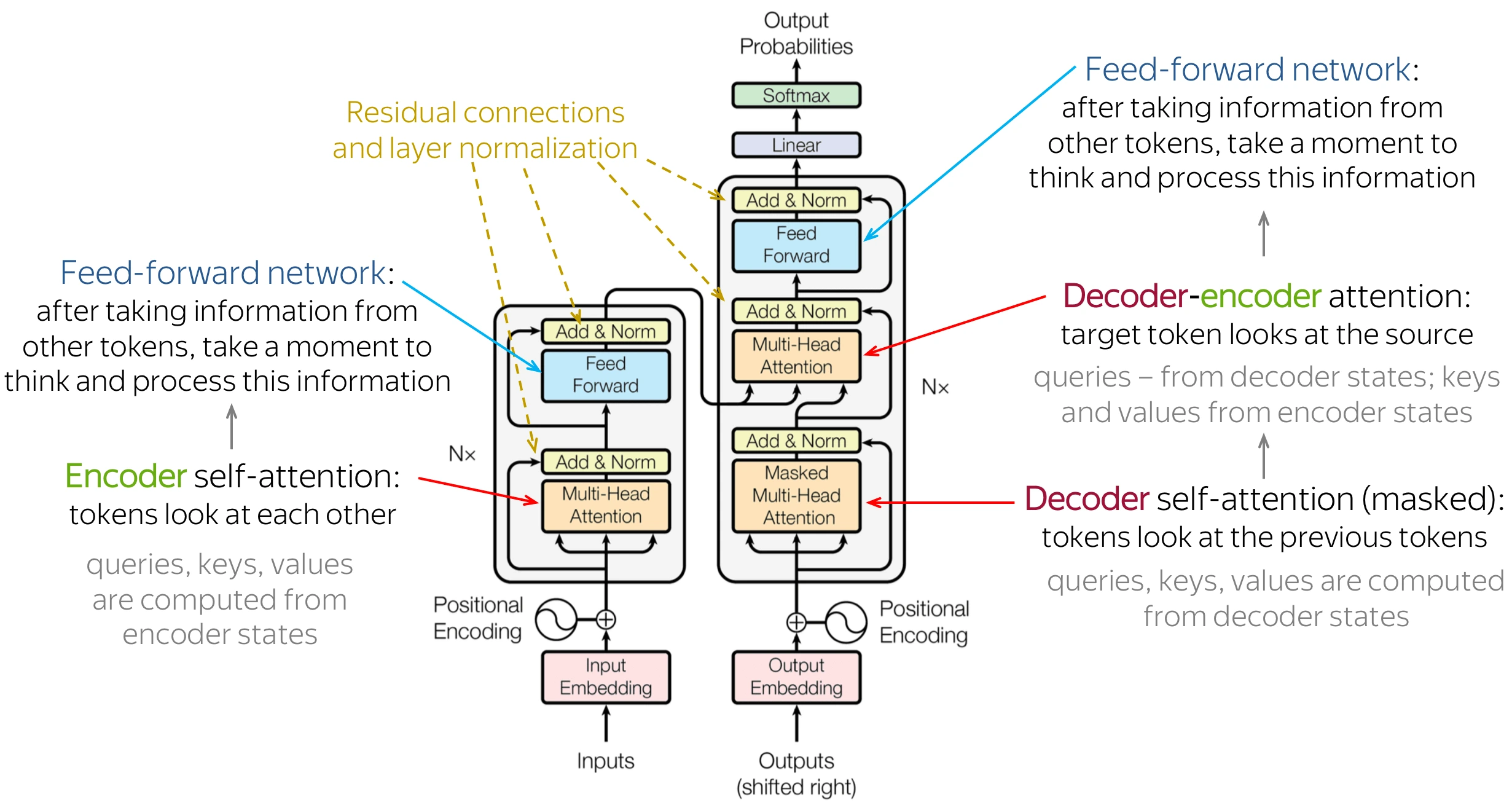
Diagram source: transformer-model-in-PyTorch, based on the original Transformer architecture from Attention Is All You Need.

Key points

< What is attention? >

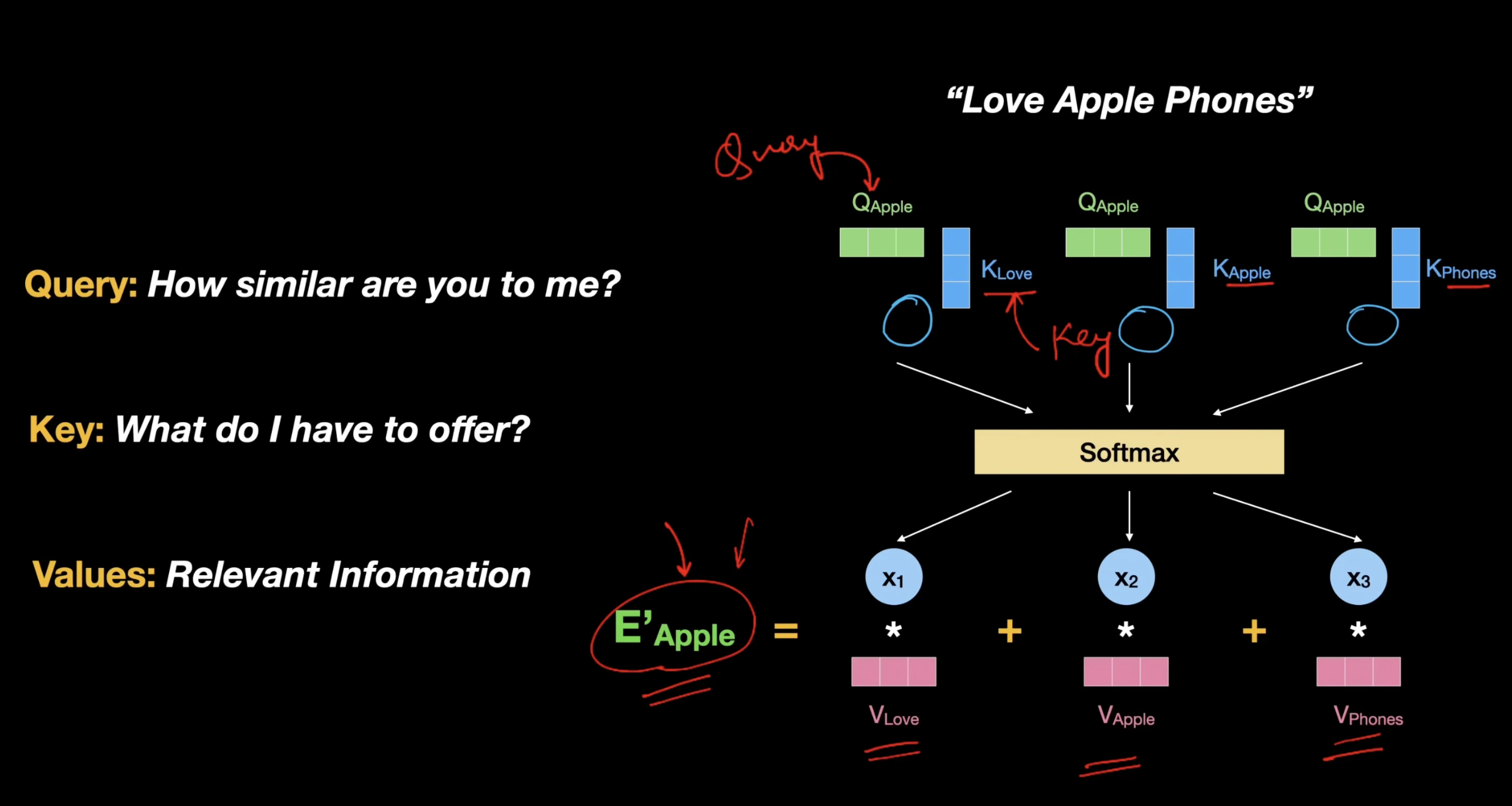
Attention is a learned way for one token to gather useful information from other tokens. For each token, the model assigns a non-negative weight to every possible source token; the weights sum to $1$. It then uses those weights to mix the source tokens' value vectors into a new, contextual representation:

$$o_i = \sum_{j=1}^{T}A_{ij}v_j$$

• Example: in “The animal rested because it was tired,” the token it can give a high weight to animal. Information from animal's value vector then becomes part of it's contextual representation.

In self-attention, the source tokens come from the same sequence. In cross-attention, they come from another sequence, such as source-language tokens in translation.

< Encoder layer and decoder layer >

The original Transformer repeats two different kinds of layers. For translation, the encoder reads the complete source sentence, while the decoder generates the target sentence one token at a time.

Layer	Main components	What it produces
Encoder layer	Self-attention over all non-padding source tokens, then a feed-forward network	A contextual representation for every source token
Decoder layer	Masked self-attention over the target prefix, cross-attention over encoder outputs, then a feed-forward network	A representation used to predict the next target token

For example, when translating “The cat sleeps.” into French, the encoder lets cat use the entire English sentence. While the decoder generates chat, its masked self-attention can use only earlier French output tokens, while cross-attention can retrieve information from English cat.

Each attention or feed-forward sublayer is wrapped in a residual connection and layer normalization. The residual path preserves the previous representation, while normalization helps the stack train stably. The $N\times$ blocks in the architecture diagram mean that these layers are repeated several times.

< Query, Key, and Value (Q, K, V) >

For a sequence representation $X$, self-attention gives every token three learned roles. The same token-representation matrix is projected into $Q$, $K$, and $V$ in parallel. The following sentence is a running example:

The animal rested because it was tired.

Lowercase $q_i$, $k_i$, and $v_i$ refer to one token's vectors. Uppercase $Q$, $K$, and $V$ refer to the matrices formed from all tokens' vectors. While the model forms the contextual representation for it, the roles are:

Symbol	Name	Intuition	Role in attention	Example
$q_i$ / $Q$	Query	What information is this token looking for?	It is compared with keys to decide where to attend	$q_{\textit{it}}$ asks which token can help explain it
$k_i$ / $K$	Key	What kind of information does this token offer?	It is matched against queries to produce attention scores	$k_{\textit{animal}}$ offers animal as a possible relevant token
$v_i$ / $V$	Value	What information should this token contribute?	It is combined using the resulting attention weights	$v_{\textit{animal}}$ provides learned context that can be mixed into it

• In the running sentence, the query for it may learn to look for a noun antecedent, while the key for animal may learn to advertise that it is one. If their score is high, softmax gives animal a high attention weight, so its value contributes strongly to it's new representation.
• In “The chef chopped the vegetables before serving them,” the query for them can similarly attend to vegetables.
• This is an intuition, not a hard-coded grammar rule: the model learns the vectors from data and can distribute attention across several tokens.

< Why use separate $Q$, $K$, and $V$? >

Queries and keys serve the matching operation, while values carry the information that is passed onward. Separate query and key projections make attention directional:

$$q_{\textit{it}}k_{\textit{animal}}^\top \ne q_{\textit{animal}}k_{\textit{it}}^\top$$

The first score can be high when it needs information from animal, without requiring the reverse score to be high. Using $QV^\top$ for matching is possible when the dimensions fit, but it forces each value vector to serve both the lookup and content roles. Distinct projections give the model more flexibility to learn what to retrieve separately from what to pass to the next layer.

< From text to $Q$, $K$, and $V$ >

The input starts as raw text. For the running example, an illustrative tokenization is:

The animal rested because it was tired.
        ↓ tokenizer
[The, animal, rested, because, it, was, tired, .]
        ↓ token embeddings + position information
x₁, x₂, x₃, x₄, x₅, x₆, x₇, x₈
        ↓ stack token vectors into X
        ↓ three learned projections, calculated in parallel
Q, K, V

Actual tokenizers may split words into subwords, so the exact token list can differ.

< Token embeddings and positions >

The tokenizer turns each token into an integer token ID. For a token at position $i$, the model retrieves its embedding from a learned embedding table $E$:

animal → token ID tᵢ → embedding-table lookup E[tᵢ] → token embedding eᵢ

$$e_i = E[t_i]$$

If the vocabulary has $|\mathcal{V}|$ tokens, $E$ has shape $(|\mathcal{V}|,d_{\mathrm{model}})$. The lookup selects one row of $E$. Mathematically, this is equivalent to multiplying a one-hot token-ID vector by $E$:

$$e_i = \operatorname{onehot}(t_i)^\top E$$

The embedding table is a learned weight matrix, but implementations normally use a fast lookup rather than explicitly multiplying a one-hot vector. During training, backpropagation updates the embedding-table rows. Later attention and MLP layers transform these initial embeddings into contextual hidden-state representations.

Here, first Transformer block means layer 1 of the Transformer stack, not the first token. It receives the initial, non-contextual token representations. Before that block, each token embedding $e_i$ is combined with position information. In a simple additive-position view:

$$x_i = e_i+p_i$$

For the first Transformer block, $X$ is the matrix of token representations:

$$X = \begin{bmatrix} x_1\\ x_2\\ \vdots\\ x_T \end{bmatrix}$$

For one sequence, $X$ has shape $(T,d_{\mathrm{model}})$. At this stage, there is one vector per token; the sequence has not been consolidated into one sentence embedding. The stack proceeds as follows:

raw text → token embeddings + positions = X⁽⁰⁾
         → Transformer block 1 → X⁽¹⁾
         → Transformer block 2 → X⁽²⁾
         → ...

In later Transformer blocks, $X$ is no longer the original token embeddings; it is the contextual hidden-state matrix output by the previous block.

Each attention head then applies three separate learned linear projections:

$$Q=XW_Q, \qquad K=XW_K, \qquad V=XW_V$$

Here, $W_Q$, $W_K$, and $W_V$ are separate learned weight matrices. The same matrix $X$ is used in all three multiplications, so the input sequence is not duplicated. For token it, the same token vector $x_{\textit{it}}$ produces three learned vectors: $q_{\textit{it}}=x_{\textit{it}}W_Q$, $k_{\textit{it}}=x_{\textit{it}}W_K$, and $v_{\textit{it}}=x_{\textit{it}}W_V$.

< Shapes in self-attention and cross-attention >

For one sequence and one attention head, omit the batch dimension and let $X$ have shape $(T,d_{\mathrm{model}})$. The projection and output shapes are:

$d_{\mathrm{model}}$ is the main hidden width of the Transformer: the number of learned numeric components in each token representation. It is not the number of tokens, layers, or vocabulary items. This width stays the same across Transformer blocks so residual connections can add their inputs and outputs. In standard multi-head attention, it is commonly divided across $h$ heads:

• Simple example: after tokenizing I like tea, suppose there are $T=3$ tokens and $d_{\mathrm{model}}=4$. The input matrix has shape $(3,4)$, so every token has four learned numeric components:

  $$X = \begin{bmatrix} 0.2 & -0.1 & 0.7 & 0.4\\ -0.3 & 0.5 & 0.1 & -0.2\\ 0.8 & 0.0 & -0.4 & 0.6 \end{bmatrix} \in\mathbb{R}^{3\times4}$$

  The rows represent I, like, and tea. The numbers are invented for illustration; a real model learns them. Every later Transformer block still receives and returns three vectors with four components each.

$$d_{\mathrm{model}} = h\cdot d_h$$

Here, $d_h$ is the head dimension: the number of learned numeric components handled by one attention head. In the common equal-width design, $d_h=d_k=d_v=d_{\mathrm{model}}/h$, so $d_{\mathrm{model}}$ must be divisible by the number of heads $h$. Heads have independent learned projections; they may learn different or overlapping attention patterns, but no linguistic role is assigned to a particular head in advance.

• Eight-head example: if $d_{\mathrm{model}}=16$ and $h=8$, then $d_h=2$. For each token, every head produces its own two-component query, key, and value vectors. For example, one head might form $q_{\textit{it}}=[0.6,-0.2]$. The two numbers are learned latent coordinates, not two named aspects of language. Each head produces its own attention pattern over the complete sequence.

Object	Shape	Role
$W_Q$	$(d_{\mathrm{model}},d_k)$	Projects a token representation into a query
$W_K$	$(d_{\mathrm{model}},d_k)$	Projects a token representation into a key
$W_V$	$(d_{\mathrm{model}},d_v)$	Projects a token representation into a value
$Q$	$(T,d_k)$	One query vector per token
$K$	$(T,d_k)$	One key vector per token
$V$	$(T,d_v)$	One value vector per token

In self-attention, all three matrices have $T$ rows because they come from the same sequence of $T$ tokens. $Q$ and $K$ must have the same vector width $d_k$ so their dot products work. $V$ may have a different width $d_v$.

• Concrete self-attention example: suppose there are $T=3$ tokens, $d_{\mathrm{model}}=12$, $d_k=7$, and $d_v=5$. Then $X$ is $(3,12)$, $W_Q$ and $W_K$ are $(12,7)$, $W_V$ is $(12,5)$, $Q$ and $K$ are $(3,7)$, and $V$ is $(3,5)$:

  $$QK^\top = (3,7)(7,3) = (3,3)$$

  The $(3,3)$ attention matrix gives one score for every query-token/key-token pair. After softmax, multiplying it by $V$ gives:

  $$AV = (3,3)(3,5) = (3,5)$$

In cross-attention, the query sequence and the key/value sequence may have different numbers of tokens. For example, 3 decoder tokens can attend to 4 encoder tokens:

$$Q:(3,7), \qquad K:(4,7), \qquad V:(4,5)$$

Then $QK^\top$ has shape $(3,4)$, and $AV$ has shape $(3,5)$. Thus, $K$ and $V$ must have the same number of rows—each key needs a corresponding value—while $Q$ can have a different number of rows.

The $W_Q$, $W_K$, and $W_V$ matrices are learned during pretraining with the rest of the model. A released checkpoint keeps them fixed during ordinary inference, while full fine-tuning can update them and adapter methods such as LoRA usually leave them frozen and learn small updates instead.

Lowercase $q_i$, $k_i$, and $v_i$ denote one token's vectors. Uppercase $Q$, $K$, and $V$ stack the corresponding vectors for all tokens, which lets the model calculate attention for the complete sequence efficiently.

< Scaled dot-product attention >

An attention score is the unnormalized compatibility score between query $q_i$ and key $k_j$. In scaled dot-product attention:

$$s_{ij} = \frac{q_i k_j^\top}{\sqrt{d_k}}$$

$d_k$ is the query and key width for one attention head: the number of learned numeric components in each vector. It is a feature width, not a token count or a number of heads. In the common equal-width design, $d_k=d_h=d_{\mathrm{model}}/h$; for $d_{\mathrm{model}}=512$ and $h=8$, $d_k=64$.

• Why divide by $\sqrt{d_k}$: if the components have similar scale, a dot product tends to grow as its dimension grows. The division keeps scores from becoming so large that softmax becomes overly peaked and gradients become less useful.

• Tiny numeric example: if $q=[2,-1,0.5]$ and $k=[1,3,4]$, each vector has three components, so $d_k=3$. Their unscaled dot product compares corresponding components:

  $$qk^\top = 2(1)+(-1)(3)+0.5(4) = 1$$

  The scaled attention score is $1/\sqrt{3}\approx0.577$.

A higher score means key $j$ is a stronger match for query $i$. Softmax converts the scores across all keys into normalized attention weights, which form a weighted sum of the values:

$$\operatorname{Attention}(Q,K,V) = \operatorname{softmax}\left(\frac{QK^\top}{\sqrt{d_k}}\right)V$$

$QK^\top$ has shape $(T,T)$: row $i$ contains how strongly token $i$ attends to every token. Some sources use “attention score” for the normalized weights too; here, it means the raw value before softmax.

• Concrete output example: In “The animal rested because it was tired,” suppose one head gives the query for it the following attention weights and two-dimensional value vectors. These are toy numbers—the real vectors are learned and usually have many more dimensions.

  Key token $j$	Attention weight $A_{\textit{it},j}$	Value vector $v_j$
  The	$0.03$	$[0.2,\;0.6]$
  animal	$0.62$	$[0.8,\;0.3]$
  rested	$0.08$	$[0.2,\;0.9]$
  because	$0.05$	$[0.4,\;1.0]$
  it	$0.12$	$[0.4,\;0.5]$
  was	$0.04$	$[0.1,\;0.6]$
  tired	$0.06$	$[0.5,\;1.0]$

  The weights sum to $1$. The output for it is their weighted mixture of value vectors:

  $$o_{\textit{it}} = \sum_j A_{\textit{it},j}v_j = [0.62,\;0.47]$$

  animal contributes the most because it has the largest weight. The output is not readable English; it is a new contextual representation of it that carries information from the tokens it attended to.

< Multi-head attention >

Multi-head attention runs $h$ independent attention projections in parallel. Each head attends over the complete sequence using its own learned $W_Q$, $W_K$, and $W_V$, so heads can learn different or overlapping patterns. Their outputs are concatenated, then $W_O$ mixes them back into the model width.

For example, if $d_{\mathrm{model}}=512$ and $h=8$, each head commonly uses $d_h=d_k=d_v=64$.

Scaled dot-product attention on the left; multiple attention heads combined on the right. Click to expand.

Diagram source: transformer-model-in-PyTorch, based on the original Transformer attention diagrams.

For head $r$, the model computes attention using its own projections, then concatenates the results from all $h$ heads:

$$\operatorname{head}_r = \operatorname{Attention}(Q_r,K_r,V_r)$$ $$\operatorname{MultiHead}(Q,K,V) = \operatorname{Concat}(\operatorname{head}_1,\ldots,\operatorname{head}_h)W_O$$

• Concrete merge: suppose $h=8$ and $d_h=2$. For token $i$, each head returns a two-number attention output:

  $$\operatorname{head}_{i,1}=[a,b], \qquad \operatorname{head}_{i,2}=[c,d], \qquad \ldots, \qquad \operatorname{head}_{i,8}=[o,p]$$

  Concatenation places the outputs side by side; it does not sum or average them:

  $$c_i = [a,b,c,d,\ldots,o,p] \in\mathbb{R}^{16}$$

  The output projection then mixes the 16 components into one updated representation for the same token:

  $$z_i = c_iW_O \in\mathbb{R}^{16}$$

  Implementations commonly calculate all heads together, then rearrange and reshape the tensor:

  (batch, heads, tokens, d_h)
  → (batch, tokens, heads, d_h)
  → (batch, tokens, heads × d_h)

  This merge happens independently at every token position, so the result is one contextual hidden-state vector per token, not one embedding for the entire sentence. A sentence-level embedding, when needed, is created later by a task-specific method such as pooling token vectors or using a special [CLS] token.

< Feed-forward network (FFN) >

After attention mixes information between tokens, a position-wise feed-forward network (FFN) transforms each token representation independently. The same FFN weights are applied at every sequence position:

$$\operatorname{FFN}(x) = W_2\,\phi(W_1x+b_1)+b_2$$

The first linear layer usually expands the representation from $d_{\mathrm{model}}$ to a larger hidden size $d_{\mathrm{ff}}$, an activation $\phi$ adds non-linearity, and the second linear layer projects it back to $d_{\mathrm{model}}$. The original Transformer used ReLU; modern models often use GELU or SwiGLU. Because the FFN does not mix positions, attention handles token-to-token communication and the FFN refines what each token has learned.

< Positional encoding >

Attention alone is permutation-equivariant: without position information, it can tell which token representations are present but not their order. Positional encoding tells the model where each token occurs in the sequence.

In the original Transformer, a position vector $p_i$ is added to each token embedding $e_i$ before the first layer, as shown earlier:

$$x_i=e_i+p_i$$

• Example: dog bites man and man bites dog contain the same words but have different meanings. Position information lets the model distinguish their order.
• Common choices: fixed sinusoidal encodings, learned position embeddings, and rotary position embeddings (RoPE). RoPE instead modifies the query and key vectors so their dot product can express relative position.

< Attention masks >

An attention mask tells a token which positions it is allowed to use. Position encoding says where a token is; a mask says which tokens it may attend to.

An attention mask $M$ is added to the raw scaled dot-product scores before softmax:

$$\operatorname{Attention}(Q,K,V;M) = \operatorname{softmax}\left( \frac{QK^\top}{\sqrt{d_k}} + M \right)V$$

$M_{ij}$ controls whether query token $i$ may attend to key token $j$. Use $0$ for an allowed position and $-\infty$ for a blocked position. After softmax, a blocked position has weight $0$. In real implementations, $-\infty$ is often represented by a very large negative number for numerical safety.

Mask	What it blocks	Example
Causal / look-ahead mask	Future keys: $j>i$	In “The cat slept,” the query at cat may attend to The and cat, but not the future token slept
Padding mask	Padding keys inserted to make a batch the same length	In a batch containing “Birds fly” and “The cat slept,” the padding after Birds fly receives no attention weight

A causal mask lets a decoder predict the next token without seeing the answer ahead of time. Padding masks prevent meaningless <PAD> tokens from affecting real token representations.

< KV cache during generation >

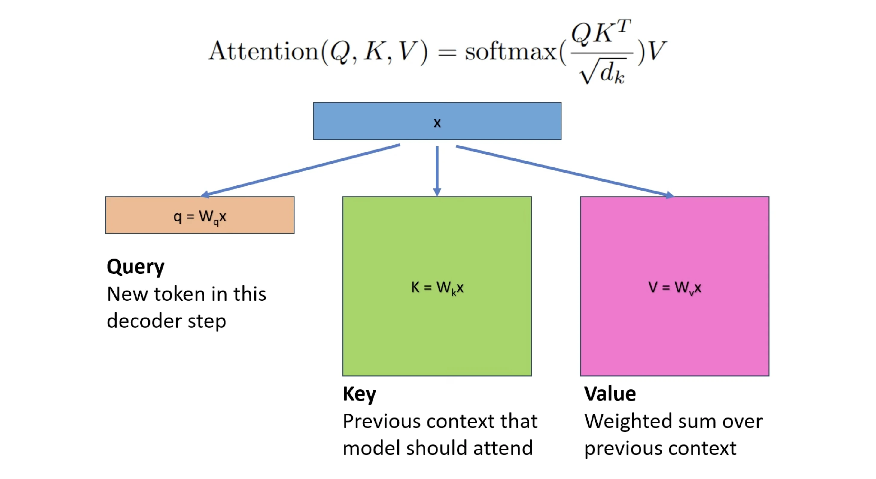
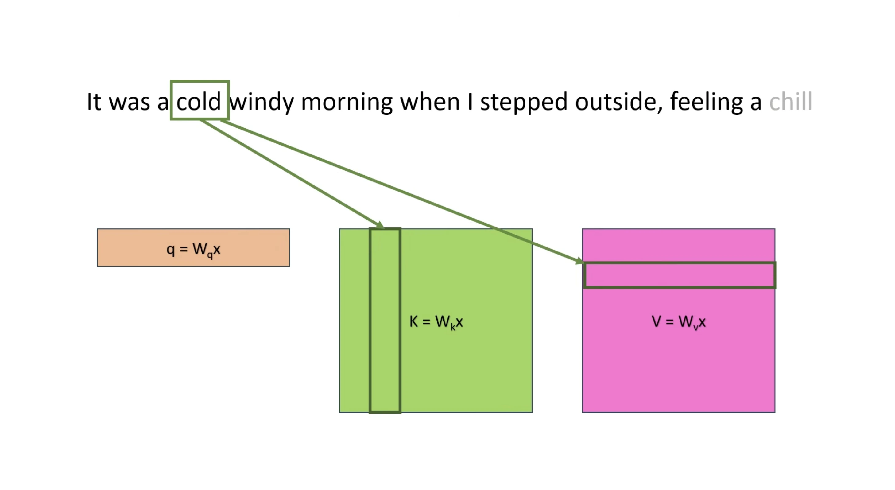
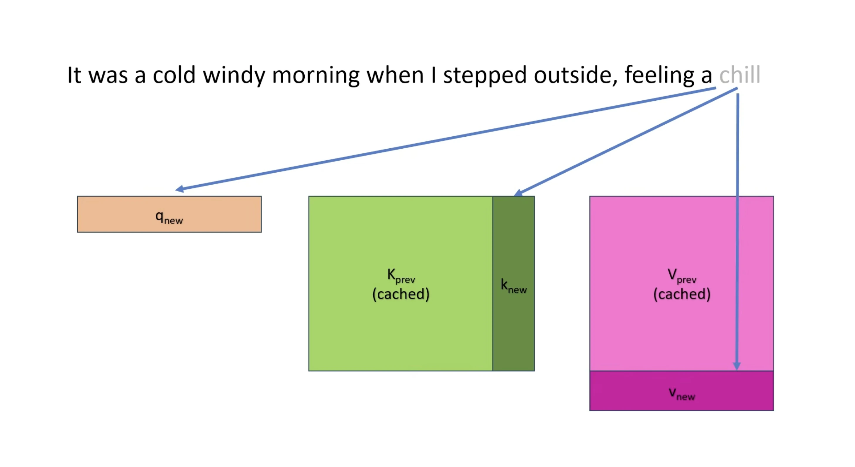
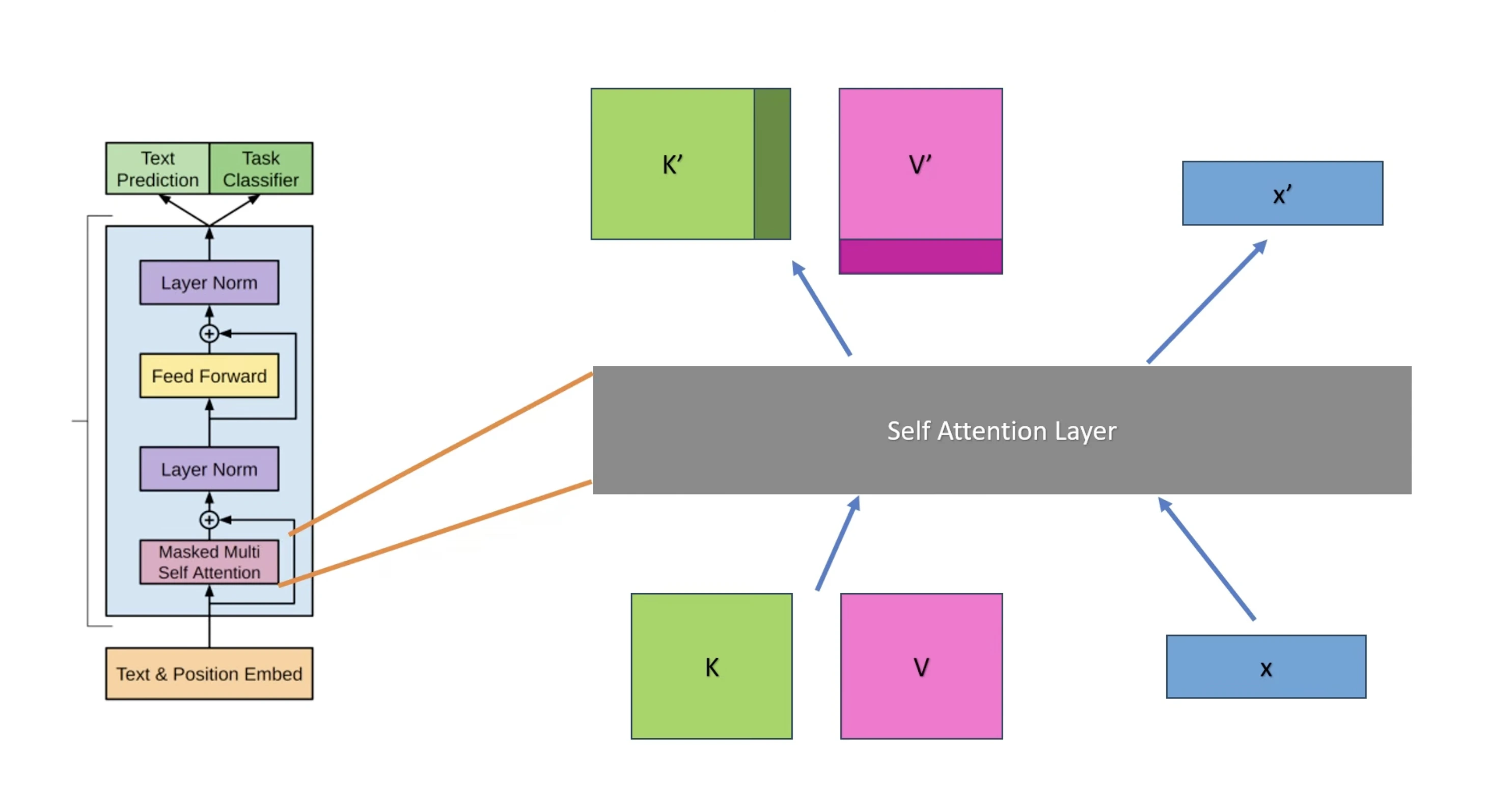
In an autoregressive decoder, a cache usually means a key–value (KV) cache. When the model generates token $t$, its new query must attend to the keys and values of all earlier tokens. Those earlier key and value vectors will not change, so the model stores them rather than recomputing the full prefix at every step.

For each layer $\ell$, the cache after processing tokens $1$ through $t-1$ contains:

$$K_{\mathrm{cache}}^{(\ell)} = \begin{bmatrix} k_1^{(\ell)}\\ \vdots\\ k_{t-1}^{(\ell)} \end{bmatrix}, \qquad V_{\mathrm{cache}}^{(\ell)} = \begin{bmatrix} v_1^{(\ell)}\\ \vdots\\ v_{t-1}^{(\ell)} \end{bmatrix}$$

• Prefill: run the prompt through every layer once and fill the cache with its $K$ and $V$ vectors.
• Decode: for the newly generated token, compute one new $q_t$, $k_t$, and $v_t$. Compare $q_t$ with the cached keys, mix the cached values, then append $k_t$ and $v_t$ to the cache.
• What it stores: numeric attention keys and values for every past token, head, and layer—commonly shaped like (batch, heads, past_length, head_dim).
• Why it stores keys and values, not queries: every later query compares with each earlier key and needs the paired value for its weighted sum. An earlier query is used only to form that earlier token's attention output, so later tokens do not need it.
• What it does not normally store: Query vectors, model weights, raw text, or verified facts. The “value” is an attention $V$ vector, not a next-token probability or the answer text.

The KV cache makes generation much faster, but it grows with sequence length and consumes memory. In an encoder–decoder model, cross-attention can also cache the encoder's keys and values because they stay fixed while the decoder generates.

KV Cache 1

KV Cache 2

KV Cache 3

KV Cache 4

Comparison

< Self-attention vs cross-attention >

Attention type	Queries come from	Keys and values come from	Typical use	Example
Self-attention	A sequence	The same sequence	Understanding relationships within text, image patches, or another sequence	In “The animal rested because it was tired,” it can attend to animal
Cross-attention	One sequence	A different sequence	A decoder attending to encoder outputs, or text attending to image features	Translate “The cat sleeps.” to “Le chat dort.”: while generating chat, the decoder can attend to source token cat

In the self-attention example, every $Q$, $K$, and $V$ vector comes from the English sentence. In the translation example, the decoder's query comes from its French-side representation, while the English encoder outputs provide the keys and values.

< Which models use an encoder or decoder? >

Model family	Encoder stack	Decoder stack	How it uses context	Typical use
BERT	✅	❌	Bidirectional self-attention over the full input	Classification, search, token representations
GPT-style	❌	✅	Causal self-attention over earlier tokens only	Text generation, chat, code completion
T5 / BART	✅	✅	Encoder reads the input; causal decoder attends to earlier output tokens and encoder output	Translation, summarization, text-to-text tasks
Vision Transformer (ViT)	✅	❌	Self-attention over image-patch tokens	Image classification and vision tasks

The words encoder and decoder describe Transformer components, not whether a model can create embeddings. A decoder-only GPT still creates useful hidden representations; it simply does so with left-to-right context rather than full bidirectional context.

Implementation

• Transformer model in PyTorch

Favorites

🤖

Magic

Related ideas

• Embeddings explains how token IDs become the vectors supplied to Transformer blocks.
• Large Language Models use Transformer-based architectures.
• Vision Transformer applies Transformer encoders to image patches.
• Low-Rank Adaptation (LoRA) adapts Transformer projections with a small number of trainable parameters.

Video Tutorial

Transformer Neural Networks, ChatGPT's foundation, Clearly Explained!!!

Attention in transformers, step-by-step | Deep Learning Chapter 6

Query, Key and Value Matrix for Attention Mechanisms in Large Language Models

Why the name Query, Key and Value? Self-Attention in Transformers

The KV Cache: Memory Usage in Transformers

Reference

• Attention Is All You Need (2017)
• Transformer using PyTorch (geeksforgeeks.org)
• LLM Visualization (by Ben Bycroft)
• Transformers Explained Visually: Learn How LLM Transformer Models Work (by Aeree, Grace, Alex, Seongmin, and Alec)
• Neural Networks - series courses (3Blue1Brown | YouTube)
• transformer-model-in-PyTorch — source of the locally copied diagrams
• Mastering LLama — Understanding Residual Connection (Hugman Sangkeun Jung)
• Attention layers in Transformer (PyLessons: architecture, code, charts, and video)