📝 Embeddings

Description

< What is it? >

An embedding is a learned dense vector that represents an input such as a text token, image patch, category, or user ID. It turns a discrete item into numbers a neural network can process. For text, the input is usually a token or subword rather than a whole word.

Key points

< How a token embedding is created >

For text, the path is:

raw text → tokenizer → token IDs → embedding-table lookup → token vectors

For example, an illustrative tokenization of “The animal rested.” is:

[The, animal, rested, .] → [t₁, t₂, t₃, t₄]

The model has a learned embedding table $E$ with one row per vocabulary token. Token ID $t_i$ selects its row:

$$e_i = E[t_i]$$

If the vocabulary contains $|\mathcal{V}|$ tokens and the model width is $d_{\mathrm{model}}$, then $E$ has shape $(|\mathcal{V}|,d_{\mathrm{model}})$. The selected row $e_i$ is the embedding vector for token $i$.

• Toy example: an embedding lookup for animal might return $e_{\textit{animal}}=[0.12,-0.41,0.77,\ldots]$. These values are learned floating-point features, not a human-readable definition of “animal.”

< Lookup versus neural-network computation >

An embedding layer is a learned weight matrix, but it normally performs a fast lookup, not a full neural-network calculation for each token. Mathematically, the lookup is equivalent to multiplying a one-hot token-ID vector by the embedding table:

$$e_i = \operatorname{onehot}(t_i)^\top E$$

During training, backpropagation updates the rows of $E$ used by the training examples. The Transformer or other neural-network layers then transform the initial embeddings into richer representations.

• Example: producing a 20-dimensional embedding with an MLP. When a Multilayer Perceptron (MLP) directly outputs an embedding, its output layer has one neuron per embedding dimension. A 20-dimensional embedding therefore comes from 20 output neurons, each producing one component of the vector:

  Hidden representation → Output layer: 20 neurons → 20-dimensional embedding
                                                    [e₁, e₂, …, e₂₀]

  If the preceding hidden layer has 64 units, the output layer in PyTorch is:

  nn.Linear(64, 20)

  Here, nn refers to torch.nn. For a batch of $B$ examples, this layer maps a hidden representation of shape $(B,64)$ to an embedding tensor of shape $(B,20)$. The 20 dimensions are learned numerical components; they do not necessarily correspond to named features such as “age” or “interest in sports.”

< Is an encoder required? >

No. A basic token embedding is already available after the embedding-table lookup; no Transformer encoder is required. A Transformer encoder is one common way to turn those initial vectors into contextual token representations:

$$H = \operatorname{Encoder}(X)$$

Desired vector	How it can be created	Need a Transformer encoder?
Initial token embedding	Lookup from the learned table $E$	No
Contextual token representation	Transformer encoder, decoder-only Transformer, RNN, or LSTM	No; an encoder is one option
Sentence embedding	Pool token vectors or use a model trained to embed complete texts	No; an encoder is often useful

A decoder-only model such as GPT has no Transformer encoder stack, but its hidden states still provide context-dependent token representations.

< Position and Transformer inputs >

A token embedding alone does not tell a Transformer where the token occurs. With additive position embeddings, the first Transformer block receives:

$$x_i = e_i+p_i$$

where $p_i$ represents position $i$. Models using rotary position embeddings (RoPE) inject position information later into queries and keys instead, but the initial token embedding still comes from the lookup table.

For a batch of text, embedding layers usually produce a tensor of shape $(B,T,d_{\mathrm{model}})$, where $B$ is batch size and $T$ is sequence length.

< Rotary position embedding (RoPE) >

Rotary Position Embedding (RoPE) encodes a token's position by rotating pairs of values in its query and key vectors. It uses an absolute position to perform the rotation, while making the attention score depend naturally on the relative distance between two tokens.

Here, $d_k$ is the number of components in each query and key vector for one attention head—not the number of tokens. It is usually even because RoPE rotates pairs of components. For example, if $d_{\mathrm{model}}=512$ is split across $8$ heads, then each head commonly has $d_k=64$. See the Transformer explanation of $d_k$.

For a query or key vector $x\in\mathbb{R}^{d_k}$ at position $p$, group adjacent values into pairs $(x_{2i},x_{2i+1})$. RoPE rotates pair $i$ by the angle $p\theta_i$:

$$\begin{bmatrix} x'_{2i}\\ x'_{2i+1} \end{bmatrix} = \begin{bmatrix} \cos(p\theta_i) & -\sin(p\theta_i)\\ \sin(p\theta_i) & \cos(p\theta_i) \end{bmatrix} \begin{bmatrix} x_{2i}\\ x_{2i+1} \end{bmatrix}$$

Here, $i=0,\ldots,d_k/2-1$. A common frequency schedule is:

$$\theta_i=10000^{-2i/d_k}$$

Each pair rotates at a different speed, allowing the model to represent both nearby and long-range position patterns.

RoPE is normally applied to queries and keys, not values:

$$\tilde q_p=R_pq_p, \qquad \tilde k_j=R_jk_j$$

The scaled attention score is then:

$$\frac{\tilde q_p^\top\tilde k_j}{\sqrt{d_k}} = \frac{q_p^\top R_p^\top R_jk_j}{\sqrt{d_k}} = \frac{q_p^\top R_{j-p}k_j}{\sqrt{d_k}}$$

The final term contains $j-p$, the relative offset between the query token at position $p$ and key token at position $j$. This is why RoPE is useful for attention: each pair of dimensions acts like a small clock hand, and the angle difference tells attention how far apart two tokens are.

< How a Transformer creates contextual embeddings >

A Transformer starts with token embeddings, then uses attention to turn them into context-aware representations. The embedding-table lookup gives the same token the same initial vector. Position information lets subsequent layers account for token order.

Each Transformer layer includes:

• Attention: each token gathers information from the tokens it is allowed to attend to. The attention mask determines which positions are available.

• Feed-forward network: transforms each token's representation.

• Residual connections and normalization: help the network train and carry information through its layers.

• Example: bank starts with the same lookup vector in “I deposited money at the bank” and “I sat beside the river bank.” After the Transformer layers, its representations can differ because the surrounding context differs.

The result is one contextual vector per token. See Transformer for the architecture and Attention Is All You Need for the original model.

< How a sentence or paragraph becomes one embedding >

A sentence embedding is one vector representing an entire piece of text. An embedding model often first creates contextual vectors for every token, then pools them into one vector:

sentence / paragraph
→ tokenizer → token IDs → initial token embeddings
→ position information + Transformer layers → contextual token vectors
→ pooling → one text embedding

For “The animal rested because it was tired,” an encoder produces one contextual vector per token:

$$H = \begin{bmatrix} h_1\\ h_2\\ \vdots\\ h_T \end{bmatrix}$$

With no padding, a simple method is mean pooling:

$$s = \frac{1}{T} \sum_{i=1}^{T}h_i$$

Here, $s$ is the sentence embedding. In practice, mean pooling excludes padding tokens. Other models use a special [CLS] token, the final valid token, or a learned pooling layer instead.

• Example: eight valid tokens with 768-dimensional contextual vectors form a tensor of shape (8, 768). Mean pooling over the token dimension produces one sentence vector of shape (768,).

Training determines whether the sentence vector is useful for similarity search. Dedicated sentence-embedding models are trained so relevant or similar texts have compatible vectors. Simply averaging an arbitrary Transformer's outputs does not guarantee this behavior; Sentence-BERT demonstrates training specifically for sentence representations.

Word2Vec produces word embeddings; a separate pooling step can combine them into a sentence embedding. Mean pooling works directly on these static word vectors, without a contextual encoder. The dimension stays the same: averaging 100-dimensional word vectors gives one 100-dimensional sentence vector, regardless of sentence length.

• Example: for “cats chase mice,” suppose the word vectors are the following illustrative values:

  Word	Word embedding
  cats	[1, 0, 1]
  chase	[0, 1, 1]
  mice	[1, 1, 0]

  The mean-pooled sentence vector is:

  $$\mathbf{s} =\frac{\mathbf{v}_{\text{cats}}+\mathbf{v}_{\text{chase}}+\mathbf{v}_{\text{mice}}}{3} =\left[\frac{2}{3},\frac{2}{3},\frac{2}{3}\right]$$

Mean pooling and TF-IDF-weighted pooling of static word vectors discard word order. Using the same Word2Vec model and consistent tokenization, sentences with the same words and occurrence counts produce the same mean-pooled embedding, up to floating-point rounding.

• Example: compare these sentence pairs, assuming usable word vectors are available:

  Sentences	Same mean-pooled embedding?
  “I love banana” / “banana love I”	Yes: the words are identical; only their order changes
  “I love banana” / “banan love I”	Not necessarily: banan is a different token and may be missing from the vocabulary

  Averaging is order-independent:

  $$\frac{v_{\text{I}}+v_{\text{love}}+v_{\text{banana}}}{3} =\frac{v_{\text{banana}}+v_{\text{love}}+v_{\text{I}}}{3}$$

These methods are useful baselines, but the averaging step itself is not trained to capture sentence meaning. A contextual sentence encoder trained for semantic similarity, such as Sentence-BERT, can represent distinctions that static averaging loses.

For a paragraph longer than an embedding model's token limit, split it into chunks and create one embedding per chunk. Retrieval systems such as RAG usually store these passage-level embeddings rather than one embedding for an entire long document.

< User embeddings and the user tower >

A user tower is the part of a recommendation model that converts information about a user into a user embedding. In a two-tower retrieval model, it is also called the query tower. The tower is the model, and the embedding is its output.

Its inputs can include a user ID, interaction history, preferences, and request context. A model using several of these inputs might process them as follows:

User ID       Recently watched movies       User preferences
   |                    |                          |
Embedding lookup   Encode / pool history     Encode features
   +--------------------+--------------------------+
                  Combine features
                         |
                  Neural network
                         |
                  User embedding
              [0.12, -0.37, ..., 0.81]

The output is a fixed-length vector, such as 128 numbers, learned to capture information useful for predicting the user's interests. Its individual dimensions do not necessarily correspond to named preferences. If the inputs include recent activity or request context, the same user can receive different embeddings as those inputs change.

• Example: a movie service can combine a learned user-ID vector with pooled embeddings of recently watched movies. The user tower transforms these features into one vector used to retrieve candidate movies.

A user tower can also be as simple as a learned user-ID embedding lookup. Additional neural-network layers are optional; the term “tower” describes the model's role in the architecture rather than a required depth.

< Two-tower scoring and training >

In a two-tower model, the user tower produces a user vector and the item tower produces an item vector of the same dimension. For dot-product retrieval, their compatibility score is:

$$\operatorname{score}(u,i) = \underbrace{f_\theta(x_u)}_{\text{user embedding}}^\top \underbrace{g_\phi(x_i)}_{\text{item embedding}}$$

Here, $x_u$ contains the user-side features, $x_i$ contains the item-side features, and $\theta$ and $\phi$ are the learned parameters of the two towers. The towers learn compatible representations in a shared embedding space; matching vector dimensions alone is not sufficient.

During training, a retrieval objective encourages observed user–item interactions to receive higher scores than sampled alternatives. Backpropagation updates both towers, including any trainable embedding tables. The embeddings therefore learn relationships relevant to the recommendation task.

At serving time, item embeddings can be precomputed and indexed. The user tower produces a query vector, and the retrieval system finds high-scoring item vectors to return as candidates. A later ranking model may refine their order. See TensorFlow's two-tower retrieval tutorial for a concrete implementation.

< Other kinds of embeddings >

• Categorical-feature embedding: a product category, country, or user ID selects a learned table row.
• Patch embedding: a Vision Transformer flattens or convolves an image patch, then projects it into a vector.
• Contextual embedding: a Transformer block turns initial token embeddings into representations that depend on the surrounding tokens.

< Word2Vec: learning static word embeddings >

Word2Vec uses a shallow neural network to learn a vector for each word from the words that appear around it. Words used in similar contexts tend to acquire similar embeddings. Google's Machine Learning Crash Course explains this context-based learning of static embeddings.

• Example: “I drink coffee every morning” and “I drink tea every morning” put coffee and tea in similar contexts. Repeated patterns like these across a corpus help shape their vectors.

Word2Vec uses self-supervised learning: the text itself supplies the training labels. A sliding context window generates input–target examples automatically, without human annotation. Training follows the familiar prediction → loss → backpropagation → weight update cycle; self-supervised describes where the labels come from.

Word2Vec has two training approaches: Continuous Bag of Words (CBOW) predicts a center word from its surrounding words; Skip-gram predicts surrounding words from the center word. The original Word2Vec paper introduces both approaches.

• Example: for the window “I love bananas,” with love as the center word:

  Model	Input	Training target
  CBOW	I, bananas	The center word: love
  Skip-gram	love	Surrounding words, through pairs: love → I and love → bananas

The training process is:

1. Create input–target examples using a sliding context window.
2. Run the forward pass to make predictions from the inputs.
3. Calculate the loss using the targets extracted from the original text.
4. Backpropagate to calculate gradients.
5. Update the weights, including the word embeddings, using an optimizer.

The training code extracts both inputs and targets when it creates each example, before the window moves. “Hiding” means leaving the target out of the prediction input; the loss function still has access to it. Moving the window creates more examples. See the TensorFlow Word2Vec tutorial for context-window pair generation and training.

Continuous Bag of Words (CBOW)

Skip-gram

Getting word embeddings

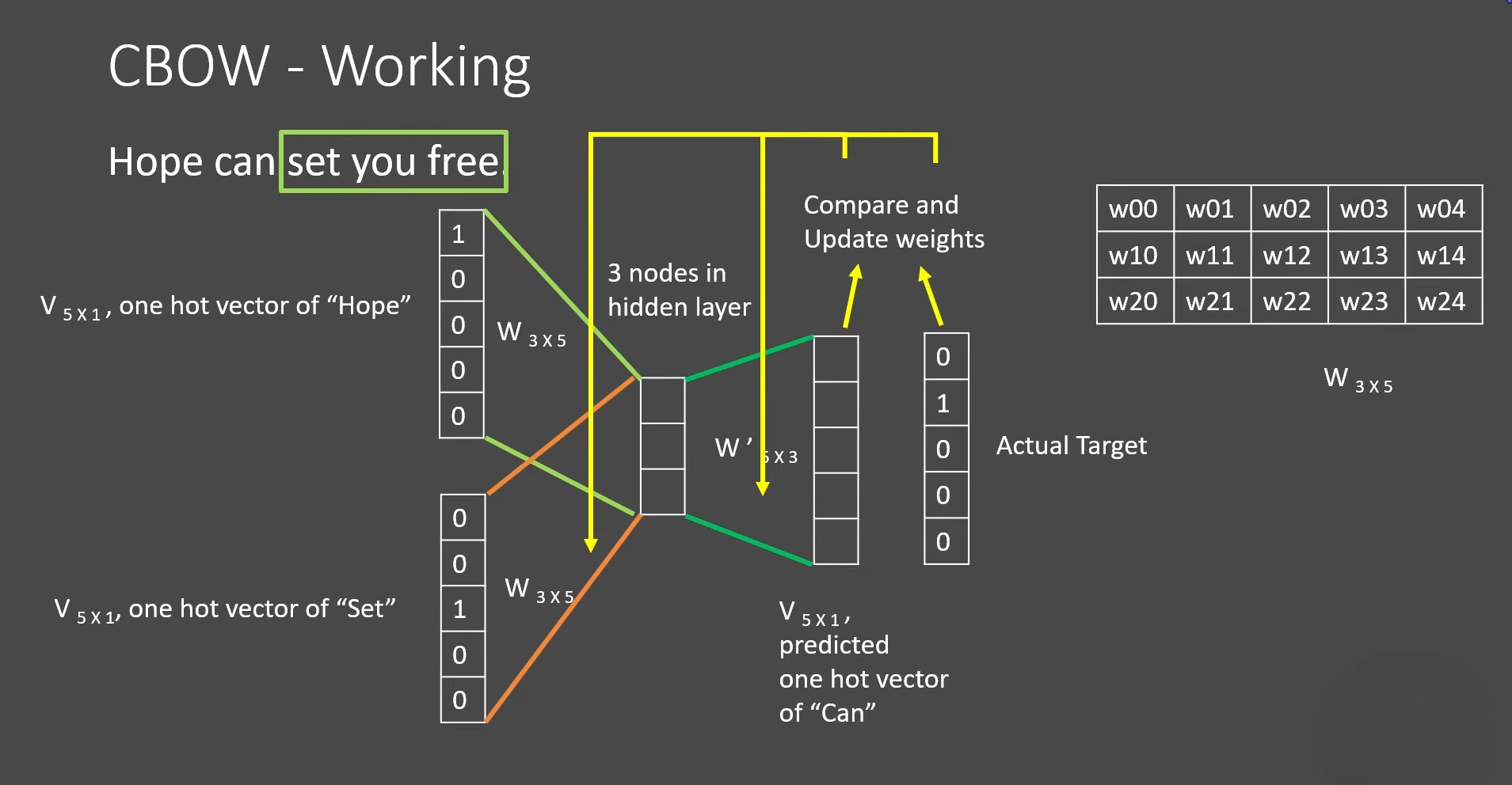
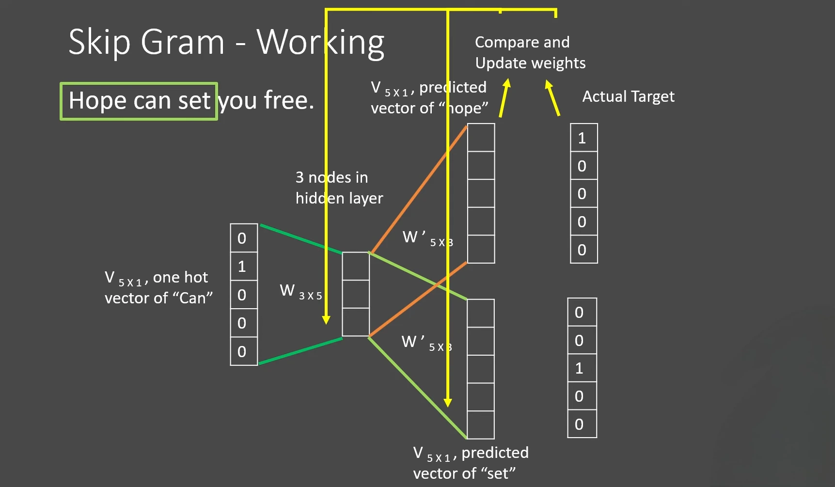
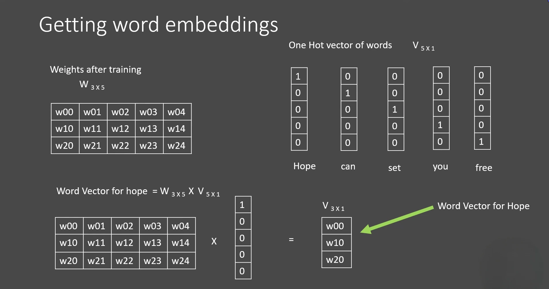
The diagrams store word vectors as columns of $W$; this is the transpose of the row-based embedding table used elsewhere on this page. For full-vocabulary prediction, output scores are converted into a probability distribution and compared with the one-hot target.

The embedding lookup is mathematically equivalent to multiplying a one-hot word vector by a learned weight matrix. The embedding projection has no nonlinear activation. Output scores feed a prediction objective, such as softmax over the vocabulary or sigmoid-based negative sampling.

• Example: the Skip-gram training path is:

  Center word ID
        ↓
  Input embedding table lookup
        ↓
  Word vector (e.g., 100 dimensions)
        ↓
  Output layer scores context words
        ↓
  Training loss updates input and output weights

Using Skip-gram with negative sampling, training works as follows:

1. Create an input embedding table. With 10,000 vocabulary words and 100-dimensional embeddings, its shape is (10000, 100). Each row starts with small random values.
2. Generate pairs and labels. A sliding context window supplies observed center–context pairs, labeled 1. Sampled noise pairs are labeled 0. These labels are generated automatically from the text and sampling procedure.
3. Run the forward pass. Look up the center word's vector. A second table holds output vectors; the dot product with each selected context-word vector produces a score.
4. Calculate the loss. A binary classification loss uses the labels to encourage higher scores for observed pairs and lower scores for sampled noise pairs. Negative sampling avoids scoring the entire vocabulary at each step.
5. Backpropagate and update the weights. Backpropagation calculates gradients, and an optimizer updates the input and output embedding weights.
6. Repeat across the corpus. Words appearing in similar contexts receive similar training signals.

• Example: one observed pair and one sampled negative might be:

  Observed pair: (cat, sits)   → encourage a higher score
  Sampled pair:  (cat, engine) → encourage a lower score

  A sampled negative is a training contrast; it does not mean those words can never occur together. The follow-up Word2Vec paper describes negative sampling.

After training, the embedding table is the useful result. A common choice is to use the input table: looking up cat returns its learned vector for similarity calculations or another model's input. Retrieving that embedding requires only a table lookup; the context-prediction output layer is no longer needed for this operation.

Word2Vec produces static embeddings: bank gets the same vector in “river bank” and “bank account.” Contextual models can produce different representations for those uses.

< GloVe: learning from global word co-occurrences >

GloVe (Global Vectors for Word Representation) learns embeddings from how often words appear near each other across a corpus. Its training targets come automatically from text, so the training can be understood as self-supervised learning, although the original work calls it unsupervised learning. See Stanford GloVe for the original material.

The training process is:

1. Count word co-occurrences. Slide a context window through the text. Build a matrix where $X_{ij}$ measures how often context word $j$ appears near word $i$, optionally weighting occurrences by their distance.

2. Initialize trainable vectors. Each word gets a word vector $w_i$, a context vector $\tilde{w}_i$, and biases $b_i$ and $\tilde{b}_i$. Choose the embedding dimension, such as 100.

3. Fit the counts. For nonzero entries, train the vectors so:

   $$w_i^\top \tilde{w}_j + b_i + \tilde{b}_j \approx \log X_{ij}$$

   A weighted squared-error loss measures the mismatch. Gradients update the vectors and biases.

4. Retrieve the embedding. After training, a common choice is:

   $$e_i = w_i + \tilde{w}_i$$

   Looking up a word returns its learned vector; no prediction pass is needed.

• Example: repeated contexts involving “drink,” “cup,” and “hot” can help coffee and tea acquire similar vectors. Each word still has one fixed embedding across sentences: GloVe produces static word embeddings.

< Other pre-Transformer methods >

Embeddings existed well before the Transformer paper in 2017. Alongside Word2Vec, earlier approaches included:

• Neural probabilistic language model (Bengio et al., 2003): learned word vectors jointly with a neural language model.
• GloVe (Pennington, Socher, and Manning, 2014): learned static vectors from global word co-occurrence statistics.

Before Transformers, RNN and LSTM language models could also create context-dependent hidden states for each token. For example, their later representation of bank could differ between “river bank” and “bank account.” Transformers made this contextual processing more parallelizable by using attention instead of recurrence.

Comparison

< Continuous Bag of Words (CBOW) vs. Skip-gram >

Approach	Input	Prediction	When to choose	Reason to choose
Continuous Bag of Words (CBOW)	Surrounding words, combined without preserving their order	The center word	Prioritize training speed, especially when processing a large corpus	Combines the context into one representation and makes one target prediction per window, usually reducing training work
Skip-gram	The center word	Surrounding words	Prioritize semantic relationships and can spend more time training	Learns from separate center–context pairs, providing individual prediction signals for neighboring words; the original paper reported stronger semantic analogy results

With four context words, CBOW makes one center-word prediction from their combined representation, while Skip-gram creates four center–context predictions. This explains the usual speed difference under comparable training settings. See the original Word2Vec paper's architecture and results sections.

Both architectures can train on small or large corpora, and both allow you to choose the embedding dimension. Larger vectors increase computation and need enough training evidence to be useful. Select the architecture and dimension by evaluating your intended task alongside training cost; the table describes tradeoffs rather than a guaranteed winner.

• Example: in “the cat sits on the mat,” use a context window of two words on each side of sits:

  CBOW:      [the, cat, on, the] → sits
  Skip-gram: sits → the
             sits → cat
             sits → on
             sits → the

  The two occurrences of the come from different positions in the window. Each center–context occurrence supplies a Skip-gram training pair.

< Word2Vec vs. GloVe >

• The core difference: Word2Vec learns through prediction tasks, while GloVe fits aggregated co-occurrence counts.

  Aspect	Word2Vec	GloVe
  Name	Word2Vec (“word to vector”)	Global Vectors for Word Representation
  Approach	Prediction-based, using a shallow neural network	Count-based, using weighted matrix factorization with biases
  Training signal	Examples drawn from local context windows across the corpus	Global co-occurrence statistics aggregated from context windows
  Created by	Google: Mikolov et al., 2013	Stanford: Pennington, Socher, and Manning, 2014
  Objective	Predict center words (CBOW) or context words (Skip-gram); negative sampling distinguishes observed pairs from noise pairs	Minimize weighted squared error between vector dot products plus biases and log co-occurrence counts
  Key idea	Learn word vectors by predicting neighboring words	Learn word vectors by fitting corpus-wide co-occurrence patterns
  Result	Static word embeddings	Static word embeddings

  Both methods derive their training signals from text. “Global” refers to GloVe's explicit aggregation of counts across the corpus; Word2Vec also learns from windows throughout the corpus. See the original Word2Vec paper and GloVe paper.

• Practical differences: compare total training cost and downstream quality under comparable settings.

  Aspect	Word2Vec	GloVe
  Training speed	Efficient training directly from context windows; cost depends on CBOW/Skip-gram, sampling, and epochs	Pays an upfront cost to build co-occurrence counts, then trains on nonzero entries; total speed depends on data and implementation
  Memory and storage	Can stream the corpus without storing a global co-occurrence matrix; still stores vocabulary and model weights	Stores co-occurrence data in addition to model weights, often increasing storage needs; RAM usage depends on buffering and implementation
  Corpus size	Supports small through very large corpora; infrequent words need enough training examples	Supports different corpus sizes; larger corpora can provide richer co-occurrence statistics, at greater preprocessing cost
  Subword information	Standard Word2Vec uses whole words; fastText is a related model that adds character n-grams	Standard GloVe uses whole words
  Tuning	Dimension, window size, learning rate, epochs, architecture, sampling, and vocabulary filtering	Dimension, window size, learning rate, iterations, vocabulary filtering, and co-occurrence weighting parameters
  Performance	Depends on corpus, settings, and downstream task	Can be comparable to Word2Vec; neither method is a universal winner

  Both methods optimize trainable vectors using gradients and vector operations. Benchmark training speed including preprocessing, and compare quality on your intended task. Implementation details: Gensim Word2Vec, Stanford GloVe, and fastText's subword representations.

• When to use which: choose based on your workflow, available data, and evaluation results.

  Consider Word2Vec when…	Consider GloVe when…
  You want a quick baseline using Gensim's built-in training API	You want ready-to-use Stanford pretrained vectors that fit your domain and vocabulary
  You want to train directly in Gensim or continue training a saved full model	You want to fit explicitly aggregated global co-occurrence statistics
  You have a small or medium corpus and want a straightforward training experiment; check that words have enough examples	You have a large corpus and resources to build and store its co-occurrence statistics
  You want to evaluate Skip-gram for infrequent words that remain in the training vocabulary	You want to evaluate whether global co-occurrence patterns improve your downstream task

  Both methods support large corpora and have pretrained vectors. Gensim can load pretrained Word2Vec and GloVe vectors. Reproducibility depends on the implementation, random seeds, data order, and parallel execution; neither method guarantees it automatically. For repeatable inference, reuse the same saved vectors and preprocessing. See Gensim's training and pretrained-model documentation and Stanford's GloVe resources.

< Profiles, towers, and embeddings >

In a recommendation system, profile describes the input data or a learned representation, while tower describes the model that processes the inputs and produces an embedding.

Concept	User side	Item side
Input profile/features	Preferences, interaction history, user ID	Category, description, item ID
Tower	Model that processes user features	Model that processes item features
Output embedding	Learned vector representing the user	Learned vector representing the item

An intuitive description is that the user tower builds a learned user profile, and the item tower builds a learned item profile, each represented as an embedding. Here, “learned profile” refers to the output vector rather than the original input features.

The precise terminology is: the user tower produces the user embedding; the item tower produces the item embedding.

< Initial, contextual, and sentence embeddings >

Aspect	Initial token embedding	Contextual token representation	Sentence embedding
Source	Direct lookup from the token ID	Output of Transformer or other neural-network layers	Pooling of word or contextual token vectors, or an encoder's sequence representation
Depends on	The token itself	The token and its surrounding context	The entire sentence or paragraph
Example	bank starts with the same embedding in every sentence	Its later vector can differ in “river bank” and “bank account”	One vector can represent “The animal rested because it was tired.”
Typical notation	$e_i$	$h_i$ or a later-layer $x_i$	$s$

< Combining word embeddings into a sentence embedding >

Method	How it works	Word order
Mean pooling of Word2Vec vectors	Average the word vectors with equal weight	Discarded
TF-IDF-weighted pooling of Word2Vec vectors	Multiply each vector by its word's TF-IDF weight, sum, and divide by the sum of weights	Discarded
Mean pooling of Transformer representations	Average the final contextual token vectors, excluding padding	Reordering words can change the vectors before averaging
Learned sequence encoder	Feed word vectors into a trained model, such as an RNN, to produce a sentence representation	Can be captured by the model

For TF-IDF weighting, use corpus statistics to compute the weights and ensure their sum is nonzero. If a word is absent from the Word2Vec vocabulary, handle it explicitly, for example by skipping it; define a fallback when no usable word vectors remain.

Implementation

< Sentence embeddings with Gensim Word2Vec >

Use Gensim to train Word2Vec, then apply mean pooling to combine word vectors into one sentence embedding. Gensim stores the learned word vectors in model.wv. Original library documentation: Gensim Word2Vec.

Install the dependencies:

python -m pip install gensim numpy

• Example: train on a small corpus and generate an embedding for “cats chase mice”:

  import numpy as np
  from gensim.models import Word2Vec
  from gensim.utils import simple_preprocess
  
  # 1. Prepare a small training corpus.
  texts = [
      "cats chase mice",
      "dogs chase cats",
      "cats and dogs are animals",
      "mice eat food",
      "dogs eat food",
  ]
  corpus = [simple_preprocess(text) for text in texts]
  
  # 2. Train word embeddings.
  model = Word2Vec(
      sentences=corpus,
      vector_size=100,  # Each word has 100 dimensions.
      window=2,
      min_count=1,
      sg=1,             # Skip-gram.
      workers=1,
      epochs=100,
      seed=42,
  )
  
  # 3. Average known word vectors into a sentence vector.
  def sentence_embedding(text):
      tokens = simple_preprocess(text)
      known_words = [word for word in tokens if word in model.wv]
  
      if not known_words:
          raise ValueError("No words from this sentence are in the vocabulary.")
  
      word_vectors = model.wv[known_words]  # Shape: (word_count, 100)
      return np.mean(word_vectors, axis=0)  # Shape: (100,)
  
  vector = sentence_embedding("cats chase mice")
  
  print("Word embedding shape:", model.wv["cats"].shape)
  print("Sentence embedding shape:", vector.shape)

  Expected output:

  Word embedding shape: (100,)
  Sentence embedding shape: (100,)

axis=0 averages each dimension across the words. Three 100-dimensional word vectors become one 100-dimensional sentence vector. Unknown words are skipped; a sentence with no known words raises an error.

This tiny corpus demonstrates the workflow. Meaningful embeddings require substantially more training text or pretrained word vectors. Mean pooling discards word order.

< Sentence embeddings with a pretrained Transformer >

The Sentence Transformers library can load a Transformer already trained for sentence embeddings. This example uses sentence-transformers/all-MiniLM-L6-v2, which produces 384-dimensional vectors. You can encode sentences without training a model yourself. See the official quickstart and the model documentation.

Install the library:

python -m pip install sentence-transformers

• Example: encode three sentences and extract the first sentence's vector:

  from sentence_transformers import SentenceTransformer
  
  # 1. Load a pretrained sentence-embedding model.
  # The first run downloads model files unless they are already cached.
  model = SentenceTransformer("sentence-transformers/all-MiniLM-L6-v2")
  
  # 2. Supply complete sentences; the model handles tokenization.
  sentences = [
      "I love bananas.",
      "Bananas are my favorite fruit.",
      "The train arrived at the station.",
  ]
  
  # 3. Generate one normalized vector per sentence.
  embeddings = model.encode(
      sentences,
      convert_to_numpy=True,
      normalize_embeddings=True,
      show_progress_bar=False,
  )
  sentence_vector = embeddings[0]
  
  print("Batch embedding shape:", embeddings.shape)
  print("Sentence embedding shape:", sentence_vector.shape)

  Expected output, excluding model download logs:

  Batch embedding shape: (3, 384)
  Sentence embedding shape: (384,)

For this model, encode() performs tokenization, Transformer processing, and mean pooling of contextual token vectors while excluding padding. normalize_embeddings=True then scales each sentence vector to unit L2 length, so its dot product with another normalized vector equals cosine similarity. You do not need to average the word vectors yourself.

Each row represents one input sentence, in the same order as sentences. The model's subword tokenizer processes the input before contextualization; it does not use the manual whole-word vocabulary filtering from the Word2Vec example.

< User and item embeddings from JSON profiles >

• Library choice: use PyTorch for numeric and categorical features and the two trainable towers, plus Sentence Transformers for the item's free-text description. Parse the JSON into fields before encoding them. Google's embedding training guide explains how task training learns useful embedding weights; PyTorch's nn.Embedding supplies categorical lookup vectors.

  Field type	Example fields	Encoding
  Numeric	Age, income, weekly watch hours, movie length	Convert units to numbers, then scale
  Single category	Gender, genre, director, company	Vocabulary ID → trainable embedding lookup
  Category list	Preferences, cast	Look up each value and mean-pool the vectors
  Free text	Short description	Pretrained Sentence Transformer → text vector
  Combined profile	All user fields or all item fields	Concatenate encoded features → MLP tower → normalized 32-dimensional vector

• Prepare valid JSON: quote keys and string values. Store units in the schema: $40k becomes 40000 in income_usd, 1h30m becomes 90 in length_minutes, and 10 hours becomes 10 in watch_hours_weekly. JSON key order has no effect because the code accesses fields by name.

• Example: generate one user vector and one item vector. Install the libraries:

  python -m pip install torch sentence-transformers

  The first run downloads the pretrained text model. The category vocabulary below is deliberately tiny; build and save it from your training data in a real system. Index 0 handles unknown categories and empty lists.

  import json
  import torch
  from torch import nn
  from torch.nn import functional as F
  from sentence_transformers import SentenceTransformer
  
  user = json.loads('''{
      "age": 15,
      "gender": "male",
      "preference": ["horror", "history", "sports"],
      "income_usd": 40000,
      "watch_hours_weekly": 10
  }''')
  item = json.loads('''{
      "genre": "horror",
      "length_minutes": 90,
      "cast": ["Jason", "David", "Michael"],
      "director": "Mike",
      "company": "Paramount",
      "short_description": "Friends investigate a haunted house."
  }''')
  
  # Field prefixes keep actor, director, and company identities separate.
  # Preferences and genres share the same topic vocabulary.
  tokens = [
      "gender:male", "topic:horror", "topic:history", "topic:sports",
      "cast:Jason", "cast:David", "cast:Michael",
      "director:Mike", "company:Paramount",
  ]
  vocab = {token: index + 1 for index, token in enumerate(tokens)}
  
  class ProfileTowers(nn.Module):
      def __init__(self, vocab, text_dim, output_dim=32):
          super().__init__()
          self.vocab = vocab
          self.category = nn.Embedding(len(vocab) + 1, 8)
          self.user_tower = nn.Sequential(
              nn.Linear(3 + 8 + 8, 64), nn.ReLU(),
              nn.Linear(64, output_dim),
          )
          self.item_tower = nn.Sequential(
              nn.Linear(1 + 4 * 8 + text_dim, 64), nn.ReLU(),
              nn.Linear(64, output_dim),
          )
  
      def category_vector(self, field, values):
          ids = [self.vocab.get(f"{field}:{value}", 0) for value in values]
          ids = torch.tensor(ids or [0], dtype=torch.long)
          return self.category(ids).mean(dim=0)
  
      def encode_user(self, profile):
          # Illustrative fixed scales; use training-data statistics in production.
          numeric = torch.tensor([
              profile["age"] / 100,
              profile["income_usd"] / 100000,
              profile["watch_hours_weekly"] / 168,
          ], dtype=torch.float32)
          features = torch.cat([
              numeric,
              self.category_vector("gender", [profile["gender"]]),
              self.category_vector("topic", profile["preference"]),
          ])
          return F.normalize(self.user_tower(features), dim=-1)
  
      def encode_item(self, profile, description_vector):
          features = torch.cat([
              torch.tensor([profile["length_minutes"] / 180],
                           dtype=torch.float32),
              self.category_vector("topic", [profile["genre"]]),
              self.category_vector("cast", profile["cast"]),
              self.category_vector("director", [profile["director"]]),
              self.category_vector("company", [profile["company"]]),
              description_vector,
          ])
          return F.normalize(self.item_tower(features), dim=-1)
  
  # This compact example runs on CPU and keeps the text encoder frozen.
  text_encoder = SentenceTransformer(
      "sentence-transformers/all-MiniLM-L6-v2", device="cpu"
  )
  description = text_encoder.encode(
      [item["short_description"]], convert_to_tensor=True,
      normalize_embeddings=True, show_progress_bar=False,
  )[0].detach().clone().float()
  
  torch.manual_seed(42)
  model = ProfileTowers(vocab, text_dim=description.numel())
  model.eval()
  with torch.no_grad():
      user_vector = model.encode_user(user)
      item_vector = model.encode_item(item, description)
      score = user_vector @ item_vector
  
  print("User embedding shape:", tuple(user_vector.shape))
  print("Item embedding shape:", tuple(item_vector.shape))
  print("Score shape:", tuple(score.shape))

  Expected output, excluding download logs:

  User embedding shape: (32,)
  Item embedding shape: (32,)
  Score shape: ()

  () means one scalar. The dot product equals cosine similarity because both vectors are normalized. The numeric score is intentionally not shown: these newly initialized towers have not learned user–item compatibility yet. Only the description encoder is pretrained.

• Train with interaction labels: a profile supplies inputs; it does not supply a target embedding. Use observed interactions, such as 1 for a clicked impression and 0 for an unclicked impression. Those labels supervise a prediction task, and gradients shape both towers' embeddings. Unclicked impressions are noisy evidence, not proof of dislike.

  Add this function after the example and call it with batches from your interaction dataset. Each row contains a user profile, an item profile, its cached description vector, and an observed label. A useful dataset includes both positive and negative examples; the single profile pair above is insufficient.

  optimizer = torch.optim.Adam(model.parameters(), lr=1e-3)
  
  def train_step(user_profiles, item_profiles, description_vectors, labels):
      model.train()
      optimizer.zero_grad()
      users = torch.stack([model.encode_user(p) for p in user_profiles])
      items = torch.stack([
          model.encode_item(p, text)
          for p, text in zip(item_profiles, description_vectors)
      ])
      # One score per observed user–item pair, scaled for the binary loss.
      logits = (users * items).sum(dim=-1) / 0.1
      targets = torch.tensor(labels, dtype=torch.float32)
      loss = F.binary_cross_entropy_with_logits(logits, targets)
      loss.backward()
      optimizer.step()
      return loss.item()

  After training, run model.eval() and encode profiles under torch.no_grad() again. Save the model weights, vocabulary, numeric preprocessing, and text-model version together. Precompute item vectors for retrieval. In this example, gradients update the categorical embeddings and both MLP towers; the cached description vectors remain fixed.

• A simpler baseline without interaction training: turn selected fields into consistent text, such as “Interested in horror, history, and sports” and “Horror movie. Friends investigate a haunted house,” then encode both with the same pretrained Sentence Transformer. This gives text-similarity vectors immediately, but numerical fields and personalized preferences are not explicitly learned. Use the structured towers when you have interaction data to train them. See the Sentence Transformers quickstart.

Video Tutorial

Word2Vect - Skipgram & CBOW

Word Embeddings: Word2Vec

GloVe

GloVe - Paper Overview

Word2Vec & GloVe

Related ideas

• Search & Retrieval combines lexical matching and semantic embedding similarity to find relevant documents.
• Term Frequency–Inverse Document Frequency (TF-IDF) represents documents using sparse term weights.
• Recommendation System explains how two-tower retrieval feeds candidate items to a ranking model.
• Transformer uses token embeddings as inputs to attention blocks.
• Vision Transformer uses embeddings for image patches.
• PyTorch is commonly used to implement embedding layers.
• Linear Algebra explains vectors and matrix multiplication.

Reference

• Sentence Transformers: Quickstart
• Sentence Transformers: all-MiniLM-L6-v2 model documentation
• Gensim: Word2Vec documentation
• Google Machine Learning Crash Course: Embeddings
• Google Machine Learning Crash Course: Embedding space and static embeddings
• Google Machine Learning Crash Course: Obtaining embeddings
• TensorFlow Recommenders: Recommending movies — retrieval
• A Neural Probabilistic Language Model
• Efficient Estimation of Word Representations in Vector Space (Word2Vec)
• Distributed Representations of Words and Phrases and their Compositionality
• Sentence-BERT: Sentence Embeddings using Siamese BERT-Networks
• word2vec (by google code)
• word2vec embeddings (gensim models word2vec)
• GloVe: Global Vectors for Word Representation
• PyTorch nn.Embedding documentation
• Attention Is All You Need
• RoFormer: Enhanced Transformer with Rotary Position Embedding