📝 Multilayer Perceptron (MLP)

Description

< What is it? >

A Multilayer Perceptron (MLP) is a feed-forward neural network made from fully connected layers, with nonlinear activations between its hidden layers. It transforms a numeric input vector into a prediction or a learned representation.

An MLP has an input, one or more hidden layers, and an output layer. Each neuron in a fully connected layer receives all values from the preceding layer. The hidden layers learn combinations of features that are useful for the training task. Google's Machine Learning Crash Course introduces these nodes and hidden layers.

Perceptron as a Linear Classifier
Linear Classifier for Complex Regions
Multi-Layer Perceptron Network

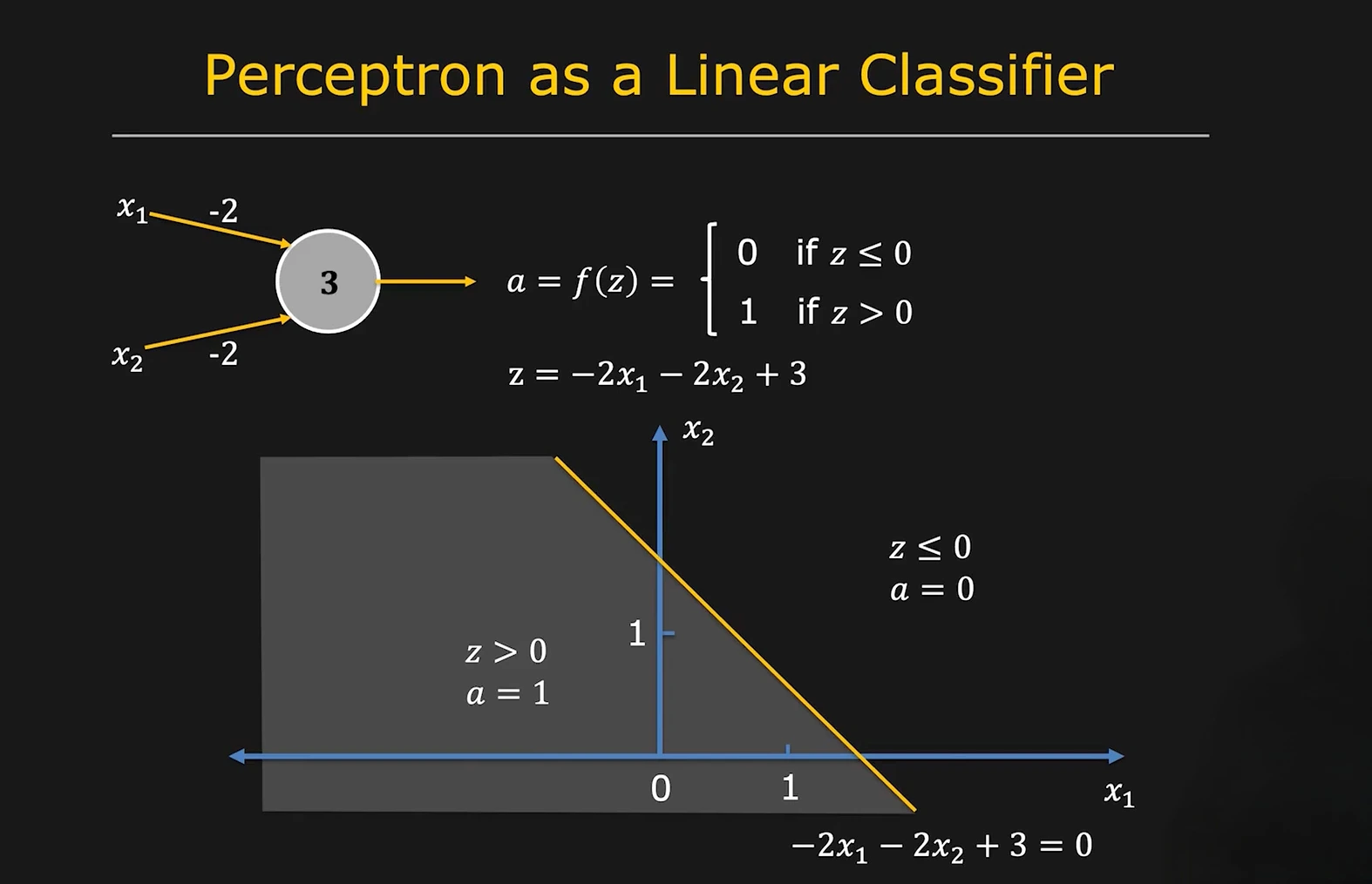
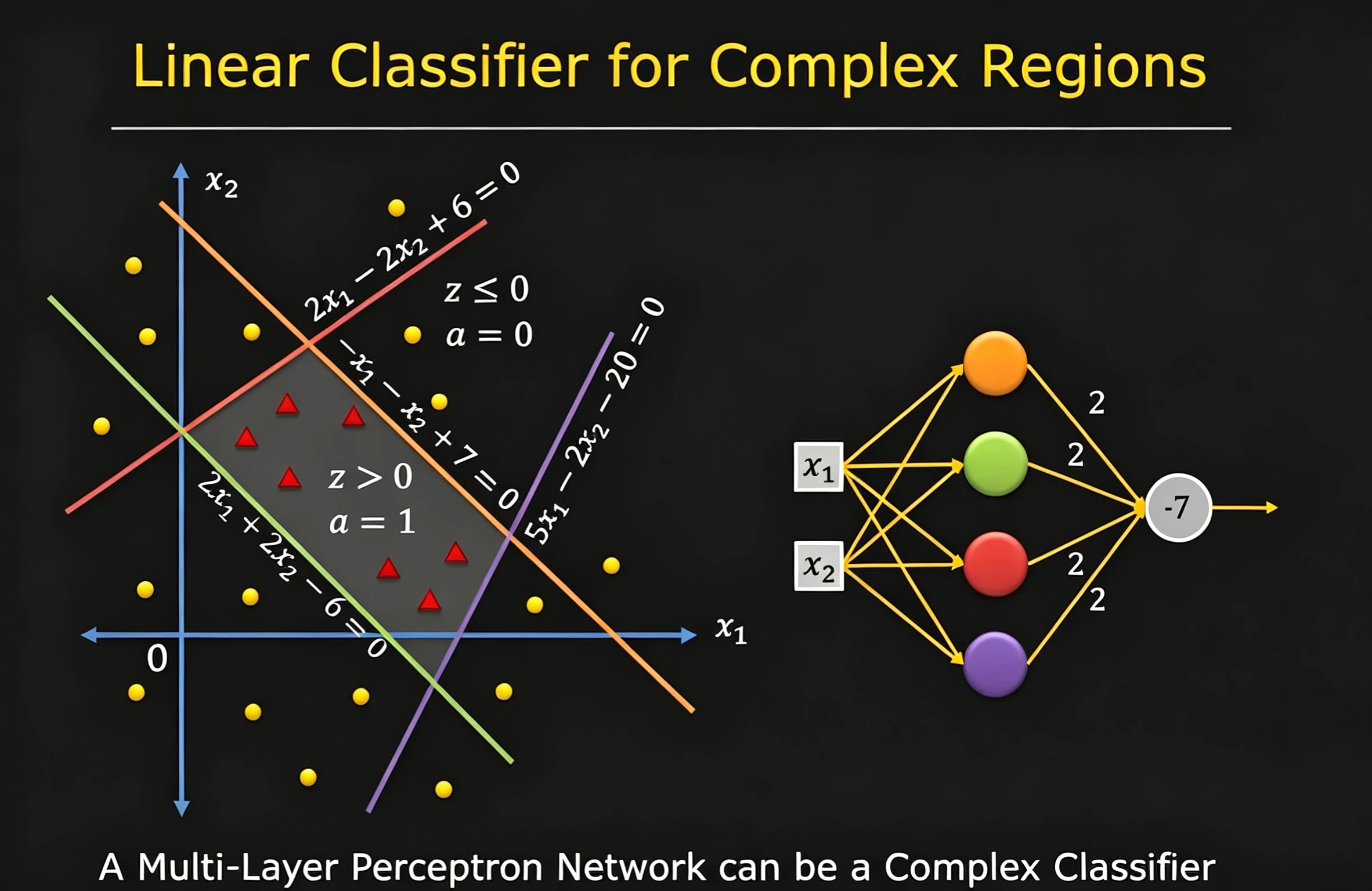
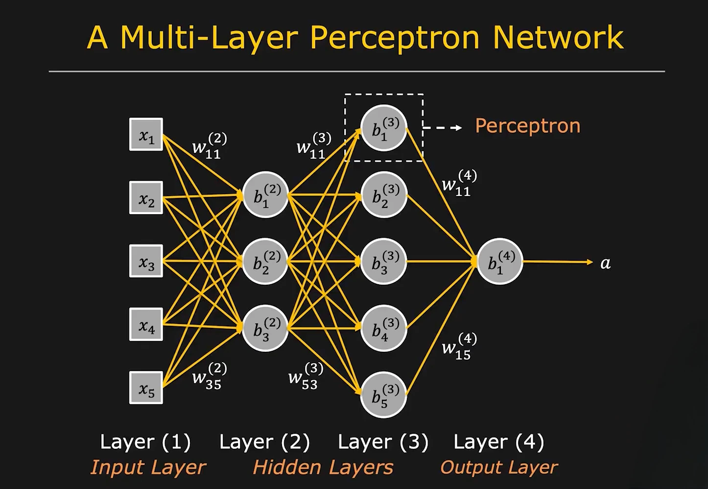
A perceptron with two inputs and a threshold activation defines a linear decision boundary.

Example: in a recommendation system, an MLP with one output neuron can learn a ranking score for each user–item pair. An MLP with $d$ output neurons can learn a $d$ -dimensional embedding for each user or item. The output size determines the shape; the training objective determines its meaning.

	Output	Label you provide	Loss	What emerges
Score / rank	1 scalar	relevance/click/rating (per item or per pair)	BCE / MSE / RankNet / LambdaRank	a sortable score
Embedding	x-dim vector	relationships (similar/dissimilar, clicked pair, class)	contrastive / triplet / InfoNCE	a metric space

So: you don't label the score or the embedding directly — you label the task or the relationships, and the score/embedding is what the network produces to satisfy that objective.

Key points

< Architecture and forward pass >

A small MLP might transform 20 input features (20 dimension embedding) through two hidden layers into one output score:

Input         Hidden layer 1      Hidden layer 2      Output
20 features → Dense(64) + ReLU → Dense(32) + ReLU → Dense(1)

Here, 20 input features means that each example is represented by a vector containing 20 numbers, so its input dimension is 20. These numbers can come from several sources:

Embedding components: one 20-dimensional embedding supplies all 20 values.
Numeric features: 20 values describing properties such as price, popularity, or interaction counts.
Combined inputs: a 16-dimensional embedding concatenated with 4 numeric features forms a 20-dimensional input vector.

A 20-dimensional embedding is therefore one possible input; the input vector can also contain ordinary numeric features or a mixture of both. For a batch of $B$ examples, the input shape is $(B,20)$ . In PyTorch, nn.Linear(20, 64) transforms each 20-dimensional input into a 64-dimensional vector, producing a tensor of shape $(B,64)$ before the activation.

Using column-vector notation, the computation is:

h_1=\operatorname{ReLU}(W_1x+b_1)

h_2=\operatorname{ReLU}(W_2h_1+b_2)

z=W_3h_2+b_3

Here, $x\in\mathbb{R}^{20}$ , $h_1\in\mathbb{R}^{64}$ , $h_2\in\mathbb{R}^{32}$ , and $z$ is a scalar. The matrices $W_1$ , $W_2$ , and $W_3$ have shapes $(64,20)$ , $(32,64)$ , and $(1,32)$ respectively. Each bias vector has the width of its layer's output.

Example: a movie ranker could receive 20 already-prepared features describing a user–movie pair and transform them into one click-prediction logit. The widths 64 and 32 are design choices, not fixed requirements.

< Nonlinear activations >

Hidden layers use activations such as the Rectified Linear Unit (ReLU), $\operatorname{ReLU}(z)=\max(0,z)$ . These allow an MLP to learn nonlinear relationships. Without nonlinearities, a stack of affine layers reduces to a single affine transformation.

The output activation depends on the task. It need not match the hidden-layer activation.

< Width, depth, and parameter count >

Width is the number of units in a layer. Depth describes the number of layers; state whether a count includes the output layer. The architecture above has two hidden layers and three trainable dense layers.

A dense layer with $n$ inputs and $m$ outputs has $nm+m$ parameters when it includes a bias. The example therefore has:

(20\times64+64)+(64\times32+32)+(32\times1+1)=3457

Increasing width or depth adds capacity and computation. Choose them using validation performance rather than assuming a larger model will generalize better. See PyTorch's Linear layer for the layer's weight and bias shapes.

< Output and training objective >

Task	MLP output	Typical training objective	Interpretation
Regression	One or more real numbers	Mean squared error	Predicted quantities
Binary classification	One logit	Binary cross-entropy with logits	Apply sigmoid for a positive-class probability
Multiclass classification	One logit per class	Cross-entropy	Apply softmax for probabilities over mutually exclusive classes
Embedding generation	A vector of a chosen dimension	Retrieval or contrastive objective	A representation trained for matching
Ranking	One score per candidate	Pointwise, pairwise, or listwise objective	Order candidates by score

Training uses a forward pass to compute outputs, a loss to measure performance, backpropagation to compute gradients, and an optimizer to update weights and biases. A hidden vector becomes useful for similarity search when training encourages the desired matching behavior.

< MLPs in recommendation systems >

An MLP can serve different roles in the same system:

User features → User MLP → User embedding ──┐
                                          ├→ Similarity → Retrieval
Item features → Item MLP → Item embedding ──┘

User embedding + item embedding + context → Ranking MLP → Score

In a retrieval tower, the MLP produces a vector, and the two towers learn compatible embeddings. In a ranking model, the MLP jointly processes user and item information to produce a score. The architecture is reusable; its inputs, output dimension, and training objective determine its role. TensorFlow demonstrates both deep retrieval towers and an MLP ranking model.

Categorical inputs can first pass through embedding lookups. A variable-length interaction history needs pooling or a sequence encoder to form a fixed-size input for a basic MLP tower.

Comparison

< Perceptron, MLP, and feed-forward network >

Term	Meaning
Perceptron	In its classical form, a linear binary classifier with a threshold decision rule
Multilayer Perceptron (MLP)	A fully connected feed-forward network with nonlinear hidden layers
Feed-forward network	A broader category in which computation flows through an acyclic graph; an MLP is one example

< MLP and XGBoost >

Aspect	MLP	XGBoost tree booster
Building blocks	Dense layers and activations	Decision trees
Training	Updates network parameters using gradients	Adds trees using loss derivatives
Representation learning	Can train embeddings and encoders jointly with a prediction head	Can consume prepared features, including embedding-derived features
Numeric preprocessing	Feature scaling often helps optimization	Standardization is generally unnecessary for tree splits
Typical role here	User/item towers or a neural ranker	A ranker over candidate feature rows

For tabular prediction, compare both on the same held-out data and task metric. An MLP is particularly convenient when the system needs to train dense representations alongside its predictions. The scikit-learn MLP guide covers training behavior and preprocessing considerations.

Implementation

< A binary classifier in PyTorch >

This runnable example trains the architecture above on synthetic data with a nonlinear label rule. It uses 768 training examples and reserves 256 examples for a final accuracy check. The fixed training duration illustrates the mechanics; real model selection should use a separate validation set.

import torch
from torch import nn

torch.manual_seed(42)
torch.set_num_threads(2)

X = torch.randn(1024, 20)
y = (X[:, 0] * X[:, 1] > 0).float().unsqueeze(1)
X_train, X_test = X[:768], X[768:]
y_train, y_test = y[:768], y[768:]

model = nn.Sequential(
    nn.Linear(20, 64),
    nn.ReLU(),
    nn.Linear(64, 32),
    nn.ReLU(),
    nn.Linear(32, 1),
)
loss_fn = nn.BCEWithLogitsLoss()
optimizer = torch.optim.Adam(model.parameters(), lr=0.01)

model.train()
for epoch in range(100):
    optimizer.zero_grad()
    logits = model(X_train)
    loss = loss_fn(logits, y_train)
    loss.backward()
    optimizer.step()

model.eval()
with torch.no_grad():
    probabilities = torch.sigmoid(model(X_test))
    predictions = (probabilities >= 0.5).float()
    accuracy = (predictions == y_test).float().mean()

print("Test accuracy:", accuracy.item())
print("Parameters:", sum(p.numel() for p in model.parameters()))

The inputs have shape (batch_size, 20) and the logits and targets have shape (batch_size, 1). BCEWithLogitsLoss combines sigmoid and binary cross-entropy in a numerically stable computation, so training passes logits directly to the loss. Sigmoid is applied explicitly when producing probabilities at inference. See the PyTorch loss documentation.

Q & A

< Is an MLP a neural network, and how do I build one in PyTorch? >

An MLP is a specific type of neural network: a feed-forward network built from fully connected layers, with nonlinear activations between them. Neural networks also include other architectures, such as convolutional networks, recurrent networks, and Transformers.

PyTorch's torch.nn provides building blocks for these architectures. To create an MLP, combine nn.Linear layers with activations such as nn.ReLU. The nn.Sequential container connects the layers in order.

Example: an MLP with 20 input features, one hidden layer of 64 neurons, and one output neuron:

from torch import nn

mlp = nn.Sequential(
    nn.Linear(20, 64),  # 20 input features → 64 hidden neurons
    nn.ReLU(),         # Nonlinear activation
    nn.Linear(64, 1),  # 64 hidden values → 1 output
)

For a batch of $B$ examples, this model maps an input of shape $(B,20)$ to an output of shape $(B,1)$ . The code creates the model; training it requires data, a loss function, and an optimizer. See PyTorch's documentation for Linear and Sequential.

A concise description is: an MLP is a fully connected feed-forward neural network that can be built using PyTorch's torch.nn components.

< How does an MLP with one output neuron learn a ranking score, and what training labels does it need? >

The output neuron produces one scalar per candidate. The target and loss give that scalar its meaning: it can predict a rating, estimate engagement, or express relative relevance. At inference, candidates for the same query or recommendation request are sorted by their scores.

(a) Pointwise — easiest

Label: a per-item target. E.g. clicked ∈ {0,1}, a star rating ∈ {1..5}, a relevance grade ∈ {0,1,2,3}, or purchase ∈ {0,1}.
Loss: BCE (if binary) or MSE (if continuous).
How it becomes a score: the raw output (a logit, or the predicted probability) is the score — you just sort items by it at inference.

Example: an item shown to a user receives label 1 if clicked and 0 otherwise. The following PyTorch snippet assumes prepared feature rows X, a one-output MLP named scorer, and floating-point labels clicked of shape (B, 1):

import torch.nn.functional as F

scores = scorer(X)  # (B, 1): one logit per user–item pair
loss = F.binary_cross_entropy_with_logits(scores, clicked)
# At inference, sort candidates for each request by descending score.

(b) Pairwise — better for ranking

Label: which of two items is more relevant for the same query. Label = 1 if item A should rank above B, else 0. (You derive these pairs from click logs: clicked > not-clicked.)
Loss: RankNet — BCE on the difference of scores:
```
scores_i = scorer(X_i)
scores_j = scorer(X_j)
loss = F.binary_cross_entropy_with_logits(scores_i - scores_j, preferred_ij)
```
Here, all three tensors have shape (B, 1), and the preference labels are floating-point values. The same scorer processes both candidates. The implied preference probability is $\sigma(s_i-s_j)$ , so training encourages the desired relative order without prescribing absolute score values. RankNet introduces this approach.

Click logs can provide preference evidence, but an unclicked item may have been unseen or still relevant. Construct pairs with exposure and position effects in mind rather than treating every missing interaction as a confirmed negative.

(c) Listwise — strongest for search/recsys

Label: graded relevance for a whole list of items under one query, e.g. [3, 0, 1, 0, 2].
Loss: LambdaRank / LambdaMART (optimizes NDCG directly) or ListNet.

Still one scalar output per item — the loss just compares the ordering your scores produce against the ideal ordering.

See the ListNet paper.
Example: five candidates for one query have relevance grades [3, 0, 1, 0, 2]. A listwise objective encourages the scores to place more relevant items earlier; it need not force the scores to equal these grades.

LambdaRank uses pairwise score updates weighted by changes in a ranking metric such as Normalized Discounted Cumulative Gain (NDCG). LambdaMART applies this approach to boosted trees. These methods target ranking quality through surrogate updates rather than differentiating the discrete sorting metric directly. See XGBoost's ranking guide.

Summary for scoring:

output = 1 scalar.
Label = a relevance/engagement signal (click, rating, grade).
The loss (pointwise/pairwise/listwise) turns that scalar into something you can sort by.

< How does an MLP with multiple output neurons learn an embedding, and what training labels does it need? >

Here's the conceptual jump: there is no "correct embedding vector" to use as a label. You don't have a target like [0.2, -0.5, ...]. Instead you supply which items should be near or far, and the network invents the coordinates that satisfy those constraints. Main recipes:

(a) Contrastive (pairs)

Label: for a pair of inputs, similar (1) or dissimilar (0). (Source: same-user sessions, augmentations of the same image, query→clicked-doc, etc.)
Loss: pull similar pairs' vectors together, push dissimilar apart:
$\mathcal{L}_{\mathrm{pair}}=yD^2+(1-y)\max(0,m-D)^2$
Here, $D$ is the distance between embeddings, $y=1$ marks a similar pair, and $m$ is a positive margin. The snippets below assume the models and input batches are already prepared.
```
za, zb = model(a), model(b)  # Each has shape (B, d).
distance = (za - zb).norm(dim=-1)
margin = 1.0
# similar: floating-point labels of shape (B,), 1 = similar, 0 = dissimilar.
loss = (
    similar * distance.square()
    + (1 - similar) * (margin - distance).clamp_min(0).square()
).mean()
```

(b) Triplet

Label: a triple (anchor, positive, negative) — positive is "same/relevant", negative is "different". The label is the grouping, not a vector.
Loss: anchor closer to positive than to negative by a margin:
$\mathcal{L}_{\mathrm{triplet}} =\max\left(0,\lVert f(a)-f(p)\rVert_2^2 -\lVert f(a)-f(n)\rVert_2^2+m\right)$
```
za, zp, zn = model(anchor), model(positive), model(negative)
positive_distance = (za - zp).square().sum(dim=-1)
negative_distance = (za - zn).square().sum(dim=-1)
margin = 1.0
loss = (positive_distance - negative_distance + margin).clamp_min(0).mean()
```

(c) Two-tower / in-batch negatives (the industry default for retrieval)

Label: just positive pairs — e.g. (query, item the user clicked). You don't even collect negatives; every other item in the minibatch serves as a negative.

Loss: InfoNCE / softmax over similarities:

import torch
import torch.nn.functional as F

q = F.normalize(query_tower(queries), dim=-1)  # (B, d)
v = F.normalize(item_tower(items), dim=-1)     # (B, d)
temperature = 0.1
logits = (q @ v.T) / temperature              # (B, B)
# Aligned positive pairs occupy the diagonal: query i matches item i.
targets = torch.arange(q.shape[0], device=q.device)
loss = F.cross_entropy(logits, targets)

This is how embedding/retrieval models (search, recommendations, sentence encoders like SBERT, CLIP) are actually trained.

(d) Classification-as-a-proxy (the "free" embedding)

Label: ordinary class labels (dog/cat, category, next-token, etc.).
Trick: train an x-class (or big-vocabulary) classifier, then throw away the final softmax layer and use the penultimate x-dim hidden vector as the embedding.
```
Input → Encoder / MLP → d-dimensional representation → C-class prediction head
```
This is why a model trained just to classify still yields useful embeddings — the representation is a byproduct.

Summary for embeddings:

output = x-dim vector.
Label = relationships (which pairs are similar / which item was clicked / which class it belongs to), never a target vector.
The loss shapes the geometry so distances become meaningful.

Video Tutorial

The Perceptron Explained
Perceptron Network

Model Lifecycle and Deployment covers data collection, training, evaluation, deployment, and monitoring, with a PyTorch serving stack and a recommendation example.
Neural Networks explains weights, biases, and the training loop.
Feed Forward Network is the broader architecture family containing MLPs.
Activation Functions describes choices for hidden and output layers.
Embeddings explains learned vectors used as MLP inputs and outputs.
Recommendation System connects retrieval towers and ranking models.
Extreme Gradient Boosting (XGBoost) provides a tree-based alternative for tabular prediction and ranking.
Backpropagation explains how gradients are calculated.
PyTorch provides tools for implementing and training the network.

Description​

< What is it? >​

Key points​

< Architecture and forward pass >​

< Nonlinear activations >​

< Width, depth, and parameter count >​

< Output and training objective >​

< MLPs in recommendation systems >​

Comparison​

< Perceptron, MLP, and feed-forward network >​

< MLP and XGBoost >​

Implementation​

< A binary classifier in PyTorch >​

Q & A​

< Is an MLP a neural network, and how do I build one in PyTorch? >​

< How does an MLP with one output neuron learn a ranking score, and what training labels does it need? >​

< How does an MLP with multiple output neurons learn an embedding, and what training labels does it need? >​

Video Tutorial​

Related ideas​

Reference​